Qualifying is where drivers push to the absolute limit. This tutorial shows you how to analyze qualifying sessions, compare progression through Q1/Q2/Q3, and identify where time is gained or lost.
Loading qualifying data
import tif1
import pandas as pd
import matplotlib.pyplot as plt
import seaborn as sns

# Load qualifying session
session = tif1.get_session(2025, "Monaco Grand Prix", "Qualifying")
laps = session.laps
Understanding qualifying structure
Modern F1 qualifying has three segments:
- Q1: All 20 drivers, bottom 5 eliminated
- Q2: Top 15 drivers, bottom 5 eliminated
- Q3: Top 10 drivers fight for pole
# Check which laps belong to which session
print(laps["Session"].value_counts())
Finding fastest laps per driver
Get each driver’s best lap time.
# Get fastest lap per driver
fastest_laps = session.get_fastest_laps(by_driver=True)

# Sort by lap time
fastest_laps_sorted = fastest_laps.sort_values("LapTime")

# Display top 10
print(fastest_laps_sorted[["Driver", "Team", "LapTime", "Compound"]].head(10))
Visualizing the Grid
Create a visual representation of the qualifying results.
# Get top 10 for pole position battle
top_10 = fastest_laps_sorted.head(10)

# Create bar chart
plt.figure(figsize=(12, 6))
colors = [f"#{row['TeamColor']}" if pd.notna(row['TeamColor']) else "#808080"
          for _, row in top_10.iterrows()]

plt.barh(top_10["Driver"], top_10["LapTime"], color=colors)
plt.xlabel("Lap Time (s)")
plt.ylabel("Driver")
plt.title("Qualifying Results - Top 10")
plt.gca().invert_yaxis()
plt.tight_layout()
plt.show()
Progression through sessions
Analyze how drivers improved from Q1 to Q3.
# Get fastest lap per driver per session segment
progression = laps.groupby(["Driver", "Session"])["LapTime"].min().reset_index()

# Pivot to show progression
progression_pivot = progression.pivot(
    index="Driver",
    columns="Session",
    values="LapTime"
)

# Calculate improvements
if "Q1" in progression_pivot.columns and "Q2" in progression_pivot.columns:
    progression_pivot["Q1_to_Q2"] = progression_pivot["Q1"] - progression_pivot["Q2"]

if "Q2" in progression_pivot.columns and "Q3" in progression_pivot.columns:
    progression_pivot["Q2_to_Q3"] = progression_pivot["Q2"] - progression_pivot["Q3"]

print(progression_pivot.head(10))
Visualizing Progression
Show how drivers improved through the sessions.
# Filter drivers who made it to Q3
q3_drivers = progression[progression["Session"] == "Q3"]["Driver"].unique()
q3_progression = progression[progression["Driver"].isin(q3_drivers)]

# Plot progression
plt.figure(figsize=(14, 8))
for driver in q3_drivers[:10]:  # Top 10 only
    driver_data = q3_progression[q3_progression["Driver"] == driver]
    plt.plot(driver_data["Session"], driver_data["LapTime"],
             marker="o", label=driver)

plt.xlabel("Session")
plt.ylabel("Lap Time (s)")
plt.title("Qualifying Progression - Top 10 Drivers")
plt.legend(bbox_to_anchor=(1.05, 1), loc="upper left")
plt.grid(True, alpha=0.3)
plt.tight_layout()
plt.show()
Tire compound analysis
See which compounds drivers used for their fastest laps.
# Compound usage in Q3
q3_laps = laps[laps["Session"] == "Q3"]
compound_usage = q3_laps.groupby(["Driver", "Compound"]).size().reset_index(name="Count")

print(compound_usage)

# Visualize
plt.figure(figsize=(12, 6))
sns.countplot(data=q3_laps, x="Driver", hue="Compound", palette="Set2")
plt.xticks(rotation=45)
plt.title("Tire Compound Usage in Q3")
plt.tight_layout()
plt.show()
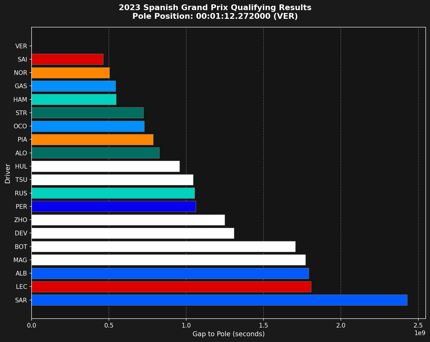
Gap to Pole
Calculate and visualize the gap to pole position.
# Get pole time
pole_time = fastest_laps_sorted["LapTime"].iloc[0]
pole_driver = fastest_laps_sorted["Driver"].iloc[0]

# Calculate gap to pole
fastest_laps_sorted["GapToPole"] = fastest_laps_sorted["LapTime"] - pole_time

# Display
print(f"Pole Position: {pole_driver} - {pole_time:.3f}s")
print("\nGap to Pole:")
print(fastest_laps_sorted[["Driver", "LapTime", "GapToPole"]].head(10))

# Visualize
plt.figure(figsize=(12, 6))
top_10_gap = fastest_laps_sorted.head(10)
plt.bar(top_10_gap["Driver"], top_10_gap["GapToPole"])
plt.xlabel("Driver")
plt.ylabel("Gap to Pole (s)")
plt.title(f"Gap to Pole Position ({pole_driver})")
plt.xticks(rotation=45)
plt.tight_layout()
plt.show()
Sector Analysis
Identify which sectors drivers are strongest in.
# Get fastest sectors per driver
sector_analysis = fastest_laps_sorted[[
    "Driver", "Sector1Time", "Sector2Time", "Sector3Time"
]].copy()

# Find fastest sector time overall
fastest_s1 = laps["Sector1Time"].min()
fastest_s2 = laps["Sector2Time"].min()
fastest_s3 = laps["Sector3Time"].min()

# Calculate delta to fastest
sector_analysis["S1_Delta"] = sector_analysis["Sector1Time"] - fastest_s1
sector_analysis["S2_Delta"] = sector_analysis["Sector2Time"] - fastest_s2
sector_analysis["S3_Delta"] = sector_analysis["Sector3Time"] - fastest_s3

print(sector_analysis.head(10))
Telemetry Comparison
Compare telemetry between pole sitter and second place.
# Get top 2 drivers
p1_driver = fastest_laps_sorted["Driver"].iloc[0]
p2_driver = fastest_laps_sorted["Driver"].iloc[1]

# Get their fastest laps
p1_fastest = session.get_driver(p1_driver).get_fastest_lap()
p2_fastest = session.get_driver(p2_driver).get_fastest_lap()

# Get telemetry
p1_tel = session.get_driver(p1_driver).get_lap(
    p1_fastest["LapNumber"].iloc[0]
).telemetry
p2_tel = session.get_driver(p2_driver).get_lap(
    p2_fastest["LapNumber"].iloc[0]
).telemetry

# Plot speed comparison
plt.figure(figsize=(14, 6))
plt.plot(p1_tel["Distance"], p1_tel["Speed"], label=p1_driver, linewidth=2)
plt.plot(p2_tel["Distance"], p2_tel["Speed"], label=p2_driver, linewidth=2)
plt.xlabel("Distance (m)")
plt.ylabel("Speed (km/h)")
plt.title("Speed Comparison - Pole vs P2")
plt.legend()
plt.grid(True, alpha=0.3)
plt.tight_layout()
plt.show()
Identifying Deleted Laps
See which laps were deleted (track limits violations).
# Filter deleted laps
deleted_laps = laps[laps["Deleted"] == True]

# Count by driver
deleted_by_driver = deleted_laps.groupby("Driver").size().sort_values(ascending=False)

print("Deleted Laps by Driver:")
print(deleted_by_driver.head(10))

# Visualize
plt.figure(figsize=(12, 6))
deleted_by_driver.head(10).plot(kind="bar")
plt.xlabel("Driver")
plt.ylabel("Number of Deleted Laps")
plt.title("Track Limits Violations")
plt.xticks(rotation=45)
plt.tight_layout()
plt.show()
Consistency Analysis
Measure driver consistency across all qualifying laps.
# Calculate standard deviation of lap times per driver
consistency = laps.groupby("Driver")["LapTime"].agg(["mean", "std", "count"])
consistency = consistency[consistency["count"] >= 3]  # At least 3 laps
consistency = consistency.sort_values("std")

print("Most Consistent Drivers:")
print(consistency.head(10))

# Visualize
plt.figure(figsize=(12, 6))
consistency.head(10)["std"].plot(kind="bar")
plt.xlabel("Driver")
plt.ylabel("Lap Time Std Dev (s)")
plt.title("Driver Consistency (Lower is Better)")
plt.xticks(rotation=45)
plt.tight_layout()
plt.show()
Complete Analysis Function
Put it all together in a reusable function.
def analyze_qualifying(year, gp):
    """Complete qualifying analysis."""
    # Load session
    session = tif1.get_session(year, gp, "Qualifying")
    laps = session.laps

    # Get fastest laps
    fastest = session.get_fastest_laps(by_driver=True).sort_values("LapTime")

    # Results
    results = {
        "pole_position": fastest.iloc[0]["Driver"],
        "pole_time": fastest.iloc[0]["LapTime"],
        "top_10": fastest.head(10)[["Driver", "Team", "LapTime"]].to_dict("records"),
        "deleted_laps": len(laps[laps["Deleted"] == True]),
        "total_laps": len(laps)
    }

    # Gap to pole
    results["gaps"] = (fastest["LapTime"] - results["pole_time"]).head(10).tolist()

    return results

# Use it
results = analyze_qualifying(2025, "Monaco Grand Prix")
print(f"Pole: {results['pole_position']} - {results['pole_time']:.3f}s")
print(f"Total laps: {results['total_laps']}, Deleted: {results['deleted_laps']}")
Summary
Qualifying analysis with tif1 allows you to:
- Identify pole position and grid order
- Track progression through Q1/Q2/Q3
- Analyze sector performance
- Compare telemetry between drivers
- Measure consistency
- Identify track limits violations
Use these techniques to understand what separates pole position from the rest of the field.
Related Pages
Race Analysis
Analyze races
Advanced Telemetry
Telemetry deep dive
Last modified on March 6, 2026