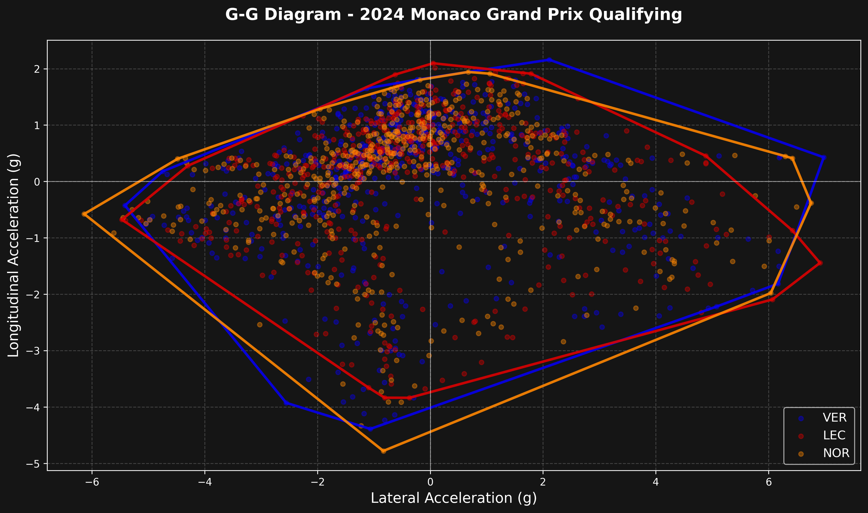
A G-G diagram plots lateral vs longitudinal acceleration, showing the performance envelope of a car. The outer boundary represents the maximum grip available - it’s one of the most insightful ways to compare car performance and driver technique.
What is a G-G diagram?
The G-G diagram shows:
- X-axis: Lateral acceleration (cornering forces)
- Y-axis: Longitudinal acceleration (braking/accelerating forces)
- Each point represents a moment in time during the lap
- The outer boundary shows the car’s performance limit
Load session and get telemetry
We’ll compare multiple drivers at Monaco Qualifying.
import math
import matplotlib.pyplot as plt
import numpy as np
from scipy.spatial import ConvexHull

import tif1
from tif1.plotting import get_team_color, setup_mpl

# Setup plotting
setup_mpl(color_scheme="fastf1")

# Load session
session = tif1.get_session(2024, "Monaco", "Q")
laps = session.laps

# Select drivers to compare
drivers = ["VER", "LEC", "NOR"]
Compute accelerations
Calculate g-forces from telemetry data using smooth derivatives to reduce noise.
The smooth_derivative() function uses a low-noise differentiator algorithm that reduces noise in the acceleration calculations. This is important because raw numerical derivatives amplify noise in the telemetry data, which would create unrealistic spikes in the G-G diagram.
def smooth_derivative(t_in, v_in):
    """Compute smooth derivative using low-noise differentiators."""
    t = t_in.copy()
    v = v_in.copy()

    # Transform time to seconds
    try:
        for i in range(0, t.size):
            t.iloc[i] = t.iloc[i].total_seconds()
    except Exception:
        pass

    t = np.array(t)
    v = np.array(v)

    dvdt = np.zeros(t.size)

    # Manually compute boundary points
    dvdt[0] = (v[1] - v[0]) / (t[1] - t[0])
    dvdt[1] = (v[2] - v[0]) / (t[2] - t[0])
    dvdt[2] = (v[3] - v[1]) / (t[3] - t[1])

    n = t.size
    dvdt[n - 1] = (v[n - 1] - v[n - 2]) / (t[n - 1] - t[n - 2])
    dvdt[n - 2] = (v[n - 1] - v[n - 3]) / (t[n - 1] - t[n - 3])
    dvdt[n - 3] = (v[n - 2] - v[n - 4]) / (t[n - 2] - t[n - 4])

    # Compute interior points with smooth method
    c = [5.0 / 32.0, 4.0 / 32.0, 1.0 / 32.0]
    for i in range(3, t.size - 3):
        for j in range(1, 4):
            dvdt[i] += 2 * j * c[j - 1] * (v[i + j] - v[i - j]) / (t[i + j] - t[i - j])

    return dvdt


def truncated_remainder(dividend, divisor):
    """Calculate truncated remainder."""
    divided_number = dividend / divisor
    divided_number = -int(-divided_number) if divided_number < 0 else int(divided_number)
    remainder = dividend - divisor * divided_number
    return remainder


def transform_to_pipi(input_angle):
    """Transform angle to [-pi, pi] range."""
    pi = math.pi
    revolutions = int((input_angle + np.sign(input_angle) * pi) / (2 * pi))
    p1 = truncated_remainder(input_angle + np.sign(input_angle) * pi, 2 * pi)
    p2 = (
        np.sign(
            np.sign(input_angle)
            + 2 * (np.sign(math.fabs((truncated_remainder(input_angle + pi, 2 * pi)) / (2 * pi))) - 1)
        )
        * pi
    )
    output_angle = p1 - p2
    return output_angle, revolutions


def remove_acceleration_outliers(acc):
    """Remove unrealistic acceleration values (> 7.5g)."""
    acc_threshold_g = 7.5
    if math.fabs(acc[0]) > acc_threshold_g:
        acc[0] = 0.0
    for i in range(1, acc.size - 1):
        if math.fabs(acc[i]) > acc_threshold_g:
            acc[i] = acc[i - 1]
    if math.fabs(acc[-1]) > acc_threshold_g:
        acc[-1] = acc[-2]
    return acc


def compute_accelerations(telemetry):
    """Calculate longitudinal and lateral accelerations in g using smooth derivatives."""
    # Longitudinal acceleration from speed change
    v = np.array(telemetry["Speed"]) / 3.6
    lon_acc = smooth_derivative(telemetry["Time"], v) / 9.81

    # Lateral acceleration from track curvature
    dx = smooth_derivative(telemetry["Distance"], telemetry["X"])
    dy = smooth_derivative(telemetry["Distance"], telemetry["Y"])

    # Calculate heading angle
    theta = np.zeros(dx.size)
    theta[0] = math.atan2(dy[0], dx[0])
    for i in range(0, dx.size):
        theta[i] = theta[i - 1] + transform_to_pipi(math.atan2(dy[i], dx[i]) - theta[i - 1])[0]

    # Curvature is rate of change of heading
    kappa = smooth_derivative(telemetry["Distance"], theta)
    lat_acc = v * v * kappa / 9.81

    # Remove outliers
    lon_acc = remove_acceleration_outliers(lon_acc)
    lat_acc = remove_acceleration_outliers(lat_acc)

    return lon_acc, lat_acc
Create G-G diagram
Plot acceleration data with performance envelope using convex hull.
The performance envelope is computed using scipy.spatial.ConvexHull, which finds the smallest convex polygon that contains all acceleration points. This accurately represents the car’s performance limits across all directions of acceleration.
fig, ax = plt.subplots(figsize=(12, 12))

for driver in drivers:
    try:
        # Get fastest lap telemetry
        driver_lap = laps.pick_driver(driver).pick_fastest()
        telemetry = driver_lap.get_telemetry().add_distance()

        # Compute accelerations
        lon_acc, lat_acc = compute_accelerations(telemetry)

        # Get team color
        try:
            team = driver_lap["Team"] if "Team" in driver_lap.index else None
            color = get_team_color(team) if team else None
        except Exception:
            color = None

        if color is None:
            # Fallback colors
            color_map = {"VER": "#0600ef", "LEC": "#dc0000", "NOR": "#ff8700"}
            color = color_map.get(driver, "#ffffff")

        # Plot scatter points
        ax.scatter(
            lat_acc,
            lon_acc,
            s=20,
            alpha=0.4,
            color=color,
            label=driver,
        )

        # Draw performance envelope using ConvexHull
        points = np.column_stack([lat_acc, lon_acc])
        points = points[~np.isnan(points).any(axis=1)]

        if len(points) > 3:
            try:
                hull = ConvexHull(points)
                # Plot the convex hull edges
                for simplex in hull.simplices:
                    ax.plot(
                        points[simplex, 0],
                        points[simplex, 1],
                        color=color,
                        linewidth=2.5,
                        alpha=0.9,
                    )
            except Exception as hull_error:
                print(f"Warning: Could not compute convex hull for {driver}: {hull_error}")
                continue

    except Exception as e:
        print(f"Warning: Could not process {driver}: {e}")
        continue

# Styling
ax.set_xlabel("Lateral Acceleration (g)", fontsize=14)
ax.set_ylabel("Longitudinal Acceleration (g)", fontsize=14)
ax.set_title(
    f"G-G Diagram - {session.event.year} {session.event['EventName']} {session.name}",
    fontsize=16,
    fontweight="bold",
    pad=20,
)

# Add grid and axis lines
ax.grid(True, alpha=0.3, linestyle="--")
ax.axhline(0, color="white", linestyle="-", alpha=0.5, linewidth=0.8)
ax.axvline(0, color="white", linestyle="-", alpha=0.5, linewidth=0.8)

# Set equal aspect ratio for proper g-force visualization
ax.set_aspect("equal")

# Legend
ax.legend(loc="lower right", fontsize=12)

plt.tight_layout()
plt.show()
Reading the diagram
Key insights from a G-G diagram:
- Top of envelope (positive Y): Maximum acceleration
- Bottom of envelope (negative Y): Maximum braking
- Left/right edges (X): Maximum cornering forces
- Corners of envelope: Combined braking/acceleration + cornering
- Wider envelope: More grip available
- Rounder envelope: Better balanced car
Comparing drivers
Look for:
- Envelope size: Larger = more grip being used
- Envelope shape: Asymmetry shows car balance issues
- Point density: Where drivers spend most time
- Peak values: Maximum g-forces achieved
Track characteristics
Different tracks produce different shapes:
- Monaco: Smaller envelope, lower speeds, less extreme forces
- Monza: Larger longitudinal values (high-speed braking)
- Silverstone: Large lateral values (high-speed corners)
The G-G diagram is a powerful tool for understanding car performance limits and how drivers extract maximum grip from the car.