Lap Time Delta Comparison

This tutorial shows how to create a lap-by-lap delta comparison between two drivers. The visualization reveals who was faster on each lap and by how much, making it easy to spot performance trends throughout a race.

Setup

import tif1
from tif1.plotting import get_team_color, setup_mpl
import matplotlib.pyplot as plt

# Setup plotting
setup_mpl(color_scheme='fastf1')

Load Session and Get Lap Data

# Load the race session
session = tif1.get_session(2024, "Monaco", "R")
laps = session.laps

# Select two drivers to compare
driver1 = "VER"
driver2 = "LEC"

# Get laps for both drivers
driver1_laps = laps[laps["Driver"] == driver1][["LapNumber", "LapTime"]].copy()
driver2_laps = laps[laps["Driver"] == driver2][["LapNumber", "LapTime"]].copy()

Calculate Time Deltas

Convert lap times to seconds and calculate the difference for each lap.

# Convert lap times to seconds
driver1_laps["LapTime"] = driver1_laps["LapTime"].dt.total_seconds()
driver2_laps["LapTime"] = driver2_laps["LapTime"].dt.total_seconds()

# Merge on lap number to compare
merged = driver1_laps.merge(
    driver2_laps,
    on="LapNumber",
    suffixes=("_d1", "_d2")
)

# Calculate delta (positive = driver2 faster, negative = driver1 faster)
merged["Delta"] = merged["LapTime_d1"] - merged["LapTime_d2"]

Color Code by Faster Driver

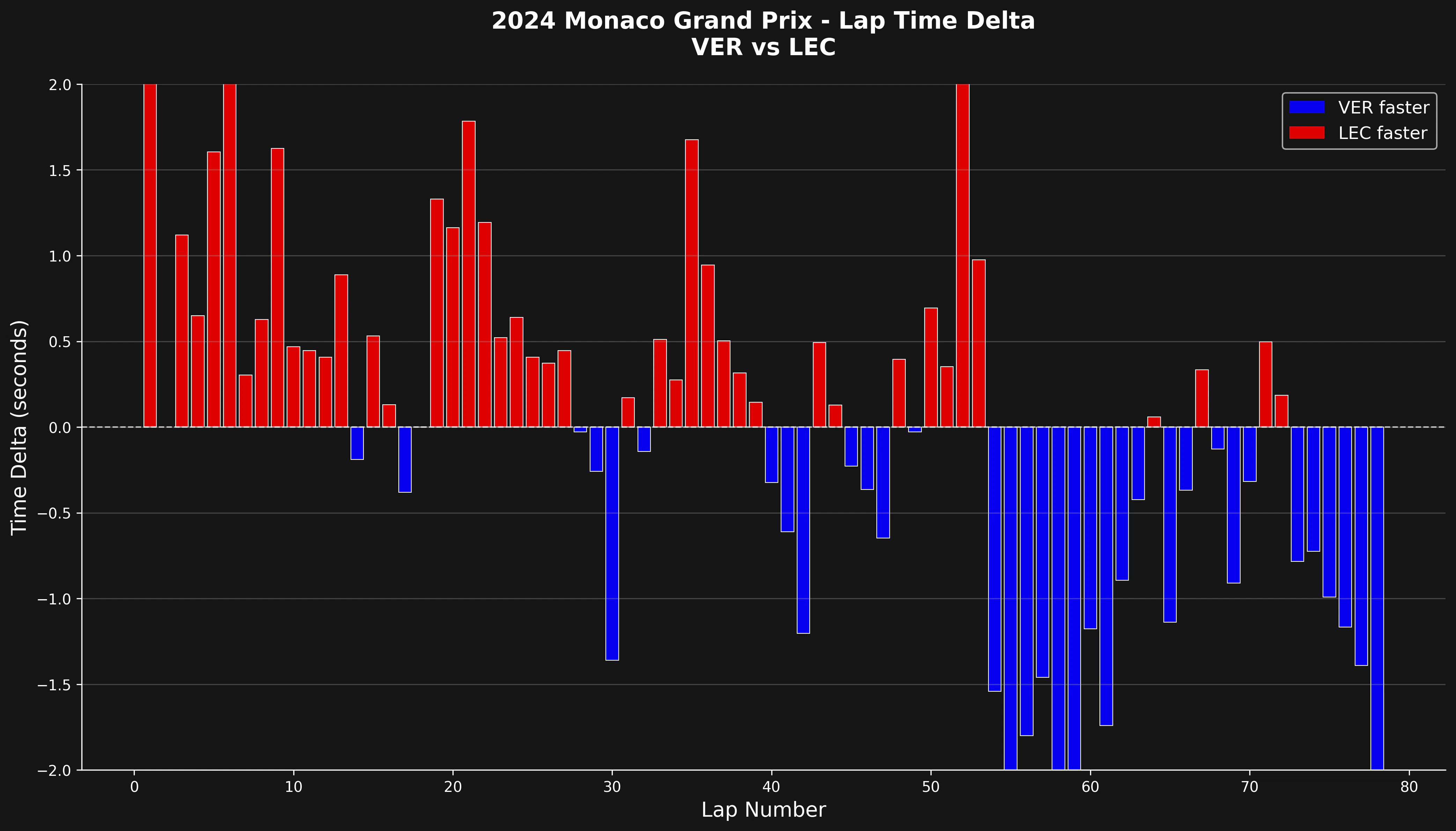
Assign colors based on which driver was faster on each lap.

# Color based on who was faster
merged["Color"] = merged["Delta"].apply(
    lambda x: get_team_color("Red Bull Racing") if x < 0
              else get_team_color("Ferrari")
)

Create the Bar Chart

Visualize the deltas with a bar chart where bar height shows the time difference.

fig, ax = plt.subplots(figsize=(14, 8))

# Bar chart of deltas
ax.bar(
    merged["LapNumber"],
    merged["Delta"],
    color=merged["Color"],
    width=0.8,
    edgecolor="white",
    linewidth=0.5,
)

# Add zero line for reference
ax.axhline(0, color="white", linestyle="--", linewidth=1, alpha=0.7)

# Labels and title
ax.set_xlabel("Lap Number", fontsize=14)
ax.set_ylabel("Time Delta (seconds)", fontsize=14)
ax.set_title(
    f"{session.event.year} {session.event['EventName']} - Lap Time Delta\n"
    f"{driver1} vs {driver2}",
    fontsize=16,
    fontweight="bold",
    pad=20,
)

Add Legend and Styling

from matplotlib.patches import Patch

# Create legend
legend_elements = [
    Patch(facecolor=get_team_color("Red Bull Racing"), label=f"{driver1} faster"),
    Patch(facecolor=get_team_color("Ferrari"), label=f"{driver2} faster"),
]
ax.legend(handles=legend_elements, loc="upper right", fontsize=12)

# Add grid and clean up
ax.grid(True, alpha=0.3, axis="y")
ax.set_ylim(-2, 2)
ax.spines["top"].set_visible(False)
ax.spines["right"].set_visible(False)

plt.tight_layout()
plt.show()

Complete Example

Here’s the full code in one block:

import matplotlib.pyplot as plt
import tif1
from tif1.plotting import get_team_color, setup_mpl
from matplotlib.patches import Patch

# Setup plotting
setup_mpl(color_scheme="fastf1")

# Load session
session = tif1.get_session(2024, "Monaco", "R")
laps = session.laps

# Select drivers
driver1 = "VER"
driver2 = "LEC"

# Get and prepare lap data
driver1_laps = laps[laps["Driver"] == driver1][["LapNumber", "LapTime"]].copy()
driver2_laps = laps[laps["Driver"] == driver2][["LapNumber", "LapTime"]].copy()

driver1_laps["LapTime"] = driver1_laps["LapTime"].dt.total_seconds()
driver2_laps["LapTime"] = driver2_laps["LapTime"].dt.total_seconds()

# Merge and calculate delta
merged = driver1_laps.merge(driver2_laps, on="LapNumber", suffixes=("_d1", "_d2"))
merged["Delta"] = merged["LapTime_d1"] - merged["LapTime_d2"]
merged["Color"] = merged["Delta"].apply(
    lambda x: get_team_color("Red Bull Racing") if x < 0
              else get_team_color("Ferrari")
)

# Create plot
fig, ax = plt.subplots(figsize=(14, 8))

ax.bar(
    merged["LapNumber"],
    merged["Delta"],
    color=merged["Color"],
    width=0.8,
    edgecolor="white",
    linewidth=0.5,
)

ax.axhline(0, color="white", linestyle="--", linewidth=1, alpha=0.7)
ax.set_xlabel("Lap Number", fontsize=14)
ax.set_ylabel("Time Delta (seconds)", fontsize=14)
ax.set_title(
    f"{session.event.year} {session.event['EventName']} - Lap Time Delta\n"
    f"{driver1} vs {driver2}",
    fontsize=16,
    fontweight="bold",
    pad=20,
)

legend_elements = [
    Patch(facecolor=get_team_color("Red Bull Racing"), label=f"{driver1} faster"),
    Patch(facecolor=get_team_color("Ferrari"), label=f"{driver2} faster"),
]
ax.legend(handles=legend_elements, loc="upper right", fontsize=12)

ax.grid(True, alpha=0.3, axis="y")
ax.set_ylim(-2, 2)
ax.spines["top"].set_visible(False)
ax.spines["right"].set_visible(False)

plt.tight_layout()
plt.show()

Interpreting the Chart

Bars above zero: Driver 2 was faster on that lap
Bars below zero: Driver 1 was faster on that lap
Bar height: Magnitude of the time difference in seconds
Color coding: Quick visual identification of who was faster

What to Look For

This visualization helps identify:

Consistency: Who maintains more consistent lap times?
Pace trends: Does one driver get faster or slower as the race progresses?
Tire degradation: Increasing deltas may indicate tire wear
Strategy impact: How do pit stops affect relative performance?
Traffic effects: Sudden spikes often indicate traffic or incidents

Filtering Out Outliers

For cleaner analysis, you can filter out pit laps and safety car periods:

# Remove pit laps
driver1_laps = driver1_laps[driver1_laps["PitOutTime"].isna()]
driver2_laps = driver2_laps[driver2_laps["PitOutTime"].isna()]

# Remove laps that are too slow (e.g., safety car)
threshold = 1.1  # 110% of fastest lap
driver1_fastest = driver1_laps["LapTime"].min()
driver2_fastest = driver2_laps["LapTime"].min()

driver1_laps = driver1_laps[driver1_laps["LapTime"] < driver1_fastest * threshold]
driver2_laps = driver2_laps[driver2_laps["LapTime"] < driver2_fastest * threshold]

Comparing Multiple Driver Pairs

You can create a function to easily compare different driver pairs:

def plot_lap_delta(session, driver1, driver2):
    """Plot lap time delta comparison between two drivers."""
    laps = session.laps

    # Get lap data
    d1_laps = laps[laps["Driver"] == driver1][["LapNumber", "LapTime"]].copy()
    d2_laps = laps[laps["Driver"] == driver2][["LapNumber", "LapTime"]].copy()

    # Convert to seconds
    d1_laps["LapTime"] = d1_laps["LapTime"].dt.total_seconds()
    d2_laps["LapTime"] = d2_laps["LapTime"].dt.total_seconds()

    # Merge and calculate delta
    merged = d1_laps.merge(d2_laps, on="LapNumber", suffixes=("_d1", "_d2"))
    merged["Delta"] = merged["LapTime_d1"] - merged["LapTime_d2"]

    # Get team colors
    d1_team = laps[laps["Driver"] == driver1].iloc[0]["Team"]
    d2_team = laps[laps["Driver"] == driver2].iloc[0]["Team"]

    merged["Color"] = merged["Delta"].apply(
        lambda x: get_team_color(d1_team) if x < 0 else get_team_color(d2_team)
    )

    # Plot
    fig, ax = plt.subplots(figsize=(14, 8))
    ax.bar(merged["LapNumber"], merged["Delta"], color=merged["Color"], width=0.8)
    ax.axhline(0, color="white", linestyle="--", linewidth=1, alpha=0.7)
    ax.set_xlabel("Lap Number")
    ax.set_ylabel("Time Delta (seconds)")
    ax.set_title(f"{driver1} vs {driver2} - Lap Time Delta")
    ax.grid(True, alpha=0.3, axis="y")

    plt.tight_layout()
    plt.show()

# Use the function
plot_lap_delta(session, "VER", "LEC")
plot_lap_delta(session, "HAM", "RUS")

Summary

Lap delta comparisons provide a clear, lap-by-lap view of relative performance between drivers. This simple visualization makes it easy to spot patterns, consistency differences, and the impact of race events on driver performance.

Driver Lap Times

Individual driver analysis

Telemetry Comparison

Detailed telemetry analysis

Race Pace Analysis

Compare race pace

Position Changes

Track position changes

Tutorials

​Setup

​Load Session and Get Lap Data

​Calculate Time Deltas

​Color Code by Faster Driver

​Create the Bar Chart

​Add Legend and Styling

​Complete Example

​Interpreting the Chart

​What to Look For

​Filtering Out Outliers

​Comparing Multiple Driver Pairs

​Summary

​Related Pages