Understanding how positions change during a race provides insights into race strategy, overtaking opportunities, and driver performance. This tutorial shows you how to create a position chart that tracks every driver’s position lap by lap.
Loading the Session
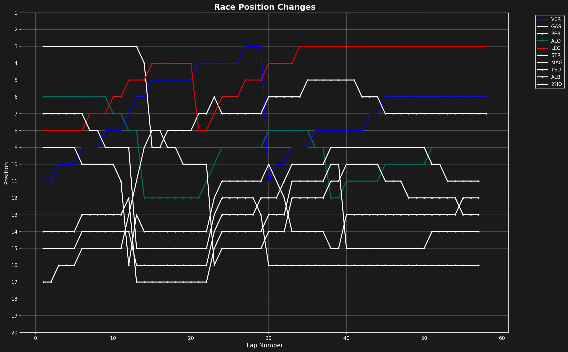
We’ll analyze the 2023 Bahrain Grand Prix, the season opener. For this visualization, we only need lap data, not telemetry or weather.
import matplotlib.pyplot as plt
import tif1

# Load the race session
session = tif1.get_session(2023, 1, "R")
laps = session.laps
Creating the Visualization
The key is to plot each driver’s position against lap number. We’ll use driver-specific colors to make the chart readable.
# Setup plotting with F1 theme
tif1.plotting.setup_mpl(mpl_timedelta_support=False, color_scheme="fastf1")

# Create the figure
fig, ax = plt.subplots(figsize=(8.0, 4.9))

# Plot each driver's position over the race
for drv in laps["Driver"].unique():
    drv_laps = laps[laps["Driver"] == drv]

    # Get driver abbreviation and color
    abb = drv_laps["Driver"].iloc[0]
    color = tif1.plotting.get_driver_color(driver=abb, session=session)

    # Plot position vs lap number
    ax.plot(drv_laps["LapNumber"], drv_laps["Position"], label=abb, color=color)
Configuring the Plot
To make the chart intuitive, we invert the y-axis so position 1 is at the top, and add appropriate labels.
# Configure axes
ax.set_ylim([20.5, 0.5])  # Invert so P1 is at top
ax.set_yticks([1, 5, 10, 15, 20])
ax.set_xlabel("Lap")
ax.set_ylabel("Position")

# Add legend outside plot area to avoid clutter
ax.legend(bbox_to_anchor=(1.0, 1.02))
plt.tight_layout()

plt.show()
Interpreting the Results
From this visualization, you can identify:
- Starting grid: Where each driver began the race
- Overtakes: Sharp position changes indicate on-track passes
- Pit stop windows: Drivers drop positions during pit stops, then recover
- Race incidents: Sudden position losses may indicate crashes or mechanical issues
- Consistent performers: Flat lines show drivers maintaining position
- Strategic gains: Gradual position improvements often indicate better strategy
Advanced: Highlighting Specific Drivers
To focus on specific drivers, you can filter the data before plotting:
# Focus on top 5 finishers
final_lap = laps[laps["LapNumber"] == laps["LapNumber"].max()]
top_5 = final_lap.sort_values("Position").head(5)["Driver"].tolist()

fig, ax = plt.subplots(figsize=(10, 6))

for drv in top_5:
    drv_laps = laps[laps["Driver"] == drv]
    abb = drv_laps["Driver"].iloc[0]
    color = tif1.plotting.get_driver_color(driver=abb, session=session)

    ax.plot(
        drv_laps["LapNumber"],
        drv_laps["Position"],
        label=abb,
        color=color,
        linewidth=2.5,
        marker="o",
        markersize=3
    )

ax.set_ylim([20.5, 0.5])
ax.set_xlabel("Lap Number")
ax.set_ylabel("Position")
ax.set_title("Top 5 Finishers - Position Changes")
ax.legend()
ax.grid(True, alpha=0.3)
plt.tight_layout()
plt.show()
Conclusion
Position change charts are essential for race analysis. They reveal the story of the race at a glance, showing strategic decisions, on-track battles, and performance trends. Combined with tire strategy and pace analysis, they provide a complete picture of race dynamics. Last modified on March 6, 2026